Graph Search, Costs, and Constraints

Driving question

A six-move shortcut crosses a one-unit gap. A detour takes fourteen moves. Which route should the robot use? You cannot answer until you know the robot's footprint and what each move costs.

Learning objectives

1. Model states, allowed moves, and edge costs.
2. Calculate f(n) = g(n) + h(n) and explain why the goal must be selected from the frontier.
3. Separate soft costs from hard feasibility constraints.
4. Check swept motion, compare search evidence, and describe the limits of a grid model.

Before, during, and after the video

Watch the full 2:04 Humanoid Hub tutorial. Every outcome is also available below and in the descriptive transcript in the Reference drawer; video playback is optional.

• Before: predict whether a 1.2-unit-wide circular robot fits a 1.0-unit gap. Explain before calculating costs.
• During: distinguish the moving search highlights from the stationary robot. Notice when actual execution begins.
• After: lower the narrow-cell penalty from twelve to two. Recalculate the small robot's choice, then ask whether the large robot's feasibility changes.

Non-video visual guide

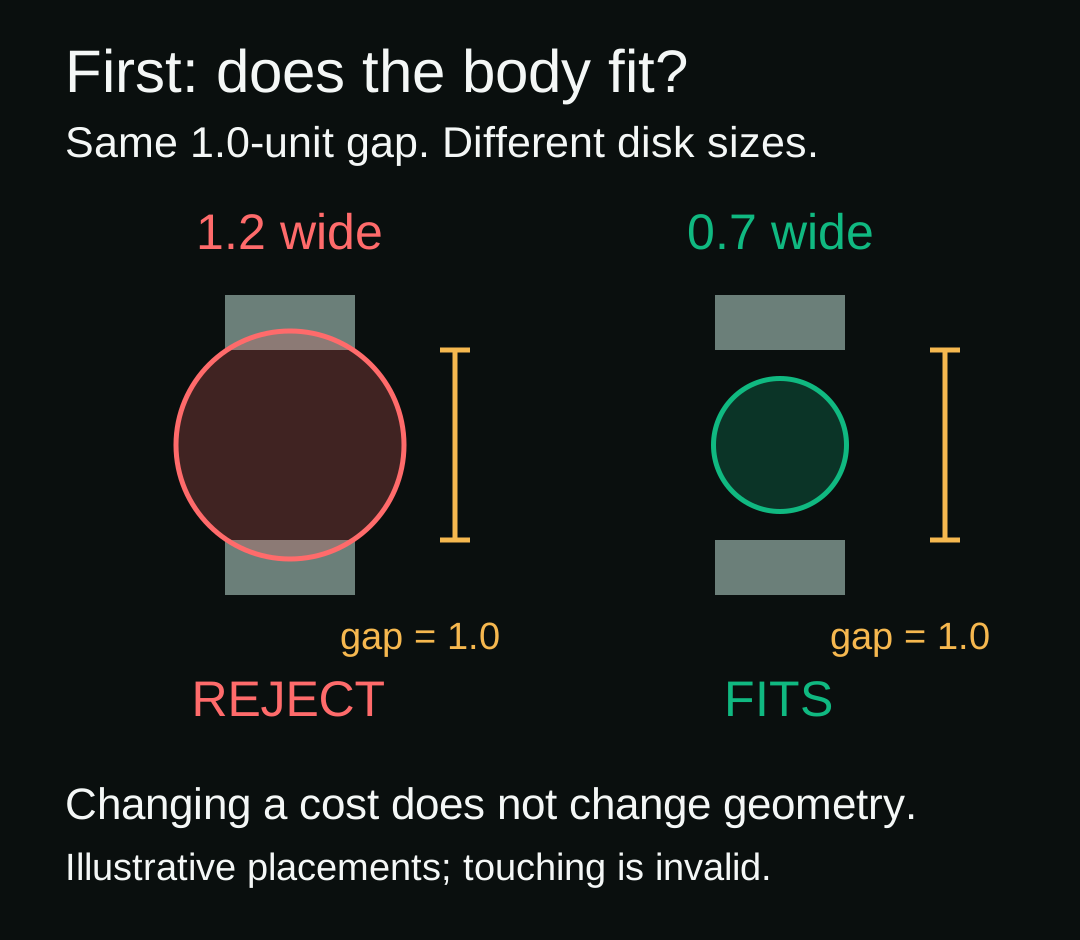
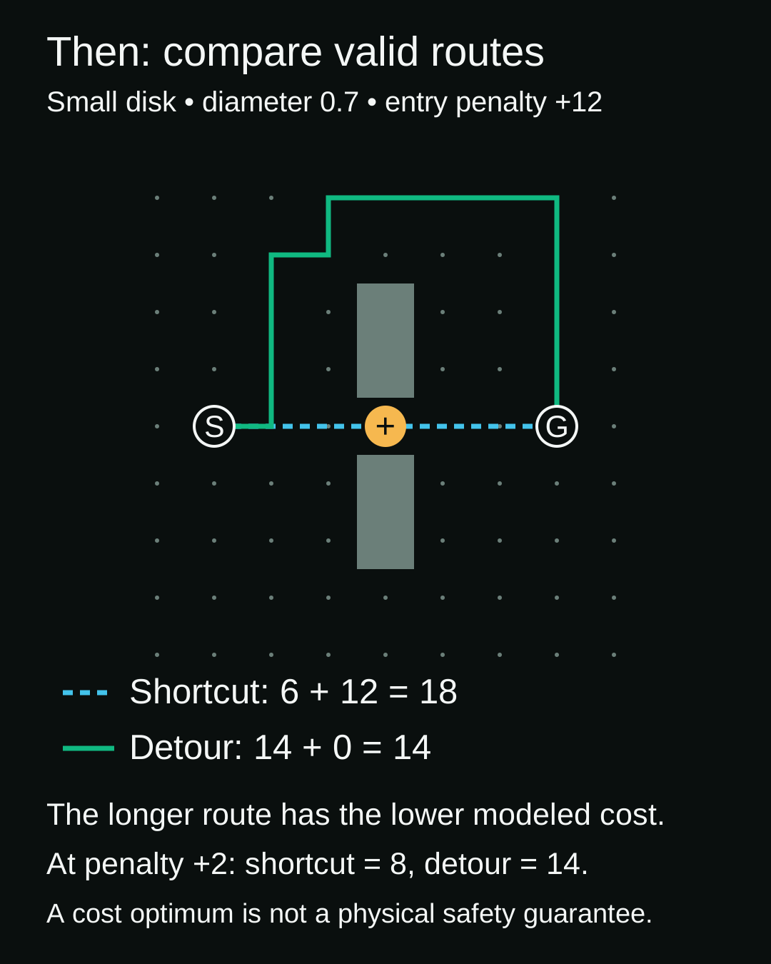
These diagrams match the worked example. The Practice lab gives the exact coordinates, arithmetic and geometry in text; no interpretation depends on color alone.

1. Define a small, honest model

Our original simulation uses integer grid centers (x,y) from 0 through 8. Start is (1,4), goal (7,4). Two rectangular obstacles occupy 3.5≤x≤4.5, with vertical intervals 1.5≤y≤3.5 and 4.5≤y≤6.5. Therefore the opening between their edges is exactly one unit. In the pictures, y increases downward.

Allowed moves are horizontal or vertical, one unit at a time. The robot is a disk that can stop and rotate in place; a car-like robot needs a different motion model. Room bounds are [-1,9]×[-1,9]. These are model units, not a recommended real robot size or clearance.

2. First decide what is possible

A point can cross the gap. A disk of radius 0.6 cannot: its diameter is 1.2, larger than the gap. Changing a cost cannot shrink the disk. Geometrically expanding an obstacle by the radius identifies forbidden center positions for this circular model. Rounded corners matter: the expansion is not an arbitrary square buffer.

Checking only waypoints is insufficient. In a negative-control test, (2,2) and (6,2) are clear but the segment between them crosses the upper obstacle. The lab rejects unsupported long jumps and separately computes segment clearance. The valid route must pass both endpoint and swept-edge tests.

Nav2's footprint guide distinguishes radius-based and polygon-based representations. Do not generalize this disk example to all robot shapes or planners.

3. Then decide which valid route is preferable

Use a smaller disk, radius 0.35 and diameter 0.7. The shortcut fits. Define each valid edge's cost as 1 + λ when its destination has obstacle/boundary clearance below 0.3; otherwise its cost is 1. Clearance means nearest obstacle/boundary distance minus the disk radius. This intentionally simple surcharge is not Nav2's inflation formula.

The six-move shortcut enters exactly one surcharged center (4,4), where clearance is 0.5−0.35=0.15. The illustrated fourteen-move detour enters none.

The detour wins under this objective, not because longer paths are intrinsically safer. If λ becomes 2, the shortcut costs 8 and wins. This changes the preference, not the collision rule. Real Nav2 inflation includes near-obstacle lethal costs as well as decaying traversal costs; “all inflation is merely a soft preference” is incorrect.

4. A* chooses what to examine next

g is the accumulated cost of the current best route to a candidate; h is a lower-bound estimate of remaining cost in the same units. A* selects the smallest f=g+h from its frontier. At (3,4) here, g=2, h=4, so f=6. The expensive gap has not yet been entered; its surcharge is added when expanding the edge into it. A low f is not a promise that this partial route will win.

For this four-neighbor model, h=|x−7|+|y−4|: at least that many unit moves remain, and every move costs at least one. Removing obstacles and nonnegative surcharges cannot make the estimate too large. The algorithm records improvements to g, skips stale queue entries and terminates when the goal is popped as the lowest-priority-value entry, not when first discovered. See Poole and Mackworth's search discussion.

The heuristic also satisfies consistency, h(u)≤c(u,v)+h(v), on every allowed edge. That supports safe graph-search pruning under these conditions; arbitrary inconsistent heuristics need more care. Consistency and pruning.

Setting h to zero gives uniform-cost search. In this exact fixture A* expands 31 nodes versus 63, both returning total 14. Ties use smaller h, then insertion order. Counts include the selected goal. These are reproducible example results, not a universal performance guarantee.

5. Keep the model's limitations visible

Finite grid optimality is not physical safety. Map freshness, localization error, stopping distance, motion dynamics and moving people are absent. Search visualization is computation; only the later execution scene depicts robot travel. A sealed passage should return NO_PATH, not disable collision checks.

Resolution also changes which geometry is represented. Smaller cells can preserve detail at greater computational cost; coarser sampling can miss obstacles or erase passages depending on occupancy aggregation. Do not claim coarsening always enlarges every obstacle. Nav2 Costmap 2D.

Retrieval check

1. Why does changing λ not let the large robot through? Geometry is a hard rejection independent of cost.
2. Why are clear endpoints insufficient? The swept edge can cross an obstacle between them.
3. If λ=2, which small-robot route wins? The shortcut: 6+2=8 versus 14.
4. What does “optimal” mean here? Lowest defined cost among allowed paths in the finite static model—not certified safety.

Summary and practice

Represent the robot. Reject invalid motion. Define cost. Search. Verify execution. Run the accessible Practice lab, explain a counterexample, then take the mastery quiz. The lesson AI assistant can provide one hint at a time without completing graded work for you.